Beyond Tradition: Harnessing Machine Learning for Demand Forecasting
In our previous article, we established robust baselines using traditional time series models like ARIMA and ETS. We validated stationarity, checked residuals, and built statistically sound forecasts. But we hit a fundamental limitation: these models only look at the past values of the series itself.
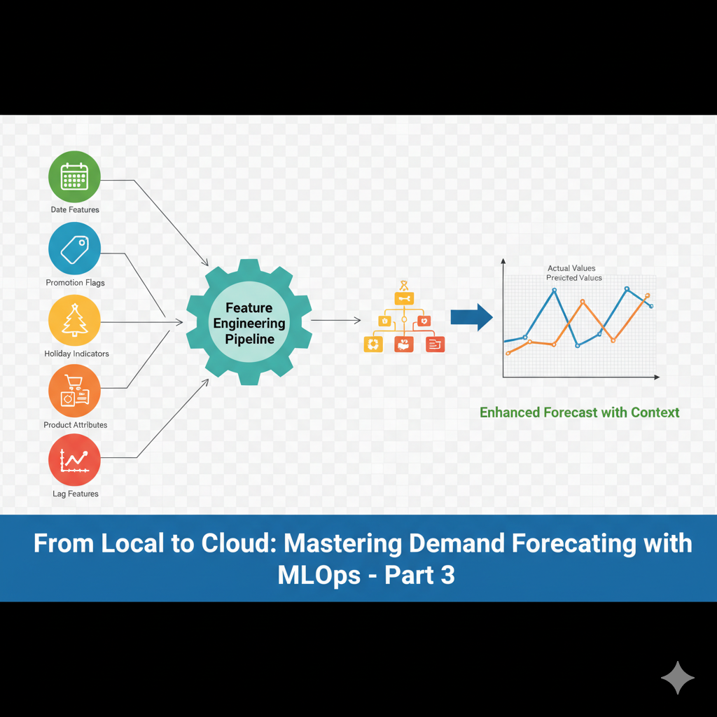
What about all the business context we simulated in our dataset? Promotions, holidays, product categories—this information is crucial for accurate demand planning. Today, we break free from tradition and harness Machine Learning to create forecasts that understand the real world.
The Power of Context: Why ML for Time Series?
Traditional models are powerful but myopic. Machine Learning models excel when we can provide them with relevant features:
- Promotions: A 30% discount will likely boost demand—this isn’t just a statistical pattern.
- Holidays: Christmas shopping behavior is fundamentally different from a random Tuesday.
- Product Categories: Electronics and clothing have completely different seasonal patterns.
- Day of Week: Weekend shopping behavior varies significantly.
Let’s enhance our single-product view from Article 2 to a multi-product, feature-rich approach.
Feature Engineering: The Real Magic
The key to successful ML for time series is thoughtful feature engineering. We’ll transform our raw data into features that help the model understand temporal patterns.
The entire code is available here: ml_time_series.ipynb
Creating Temporal Features
def create_features(df):
    df = df.copy()
    df['date'] = pd.to_datetime(df.index)

    # Basic date features
    df['day_of_week'] = df['date'].dt.dayofweek
    df['day_of_month'] = df['date'].dt.day
    df['week_of_year'] = df['date'].dt.isocalendar().week
    df['month'] = df['date'].dt.month
    df['quarter'] = df['date'].dt.quarter
    df['year'] = df['date'].dt.year
    df['is_weekend'] = (df['date'].dt.dayofweek >= 5).astype(int)

    # Cyclical encoding for periodic features
    df['day_of_week_sin'] = np.sin(2 * np.pi * df['day_of_week']/7)
    df['day_of_week_cos'] = np.cos(2 * np.pi * df['day_of_week']/7)
    df['month_sin'] = np.sin(2 * np.pi * df['month']/12)
    df['month_cos'] = np.cos(2 * np.pi * df['month']/12)

    # Holiday proximity (days until next major holiday)
    def days_to_holiday(date):
        holidays = {
            'christmas': pd.Timestamp(f'{date.year}-12-25'),
            'new_year': pd.Timestamp(f'{date.year+1}-01-01'),
            'july_4': pd.Timestamp(f'{date.year}-07-04')
        }
        min_days = 365
        for holiday in holidays.values():
            days = abs((date - holiday).days)
            min_days = min(min_days, days)
        return min_days

    df['days_to_holiday'] = df['date'].apply(days_to_holiday)

    return df

# Apply feature engineering
df_enhanced = create_features(df).reset_index(drop=True)
Creating Lag and Window Features
This is where we help the model understand recent trends and patterns.
# Create lag and rolling window features for a specific product
def create_lag_features(df, product_id, lag_periods=[1, 7, 14, 28], window_sizes=[7, 28]):
    product_df = df[df['product_id'] == product_id].copy().sort_values('date')

    # Lag features
    for lag in lag_periods:
        product_df[f'lag_{lag}'] = product_df['units_sold'].shift(lag)

    # Rolling statistics
    for window in window_sizes:
        product_df[f'rolling_mean_{window}'] = product_df['units_sold'].shift(1).rolling(window=window).mean()
        product_df[f'rolling_std_{window}'] = product_df['units_sold'].shift(1).rolling(window=window).std()
        product_df[f'rolling_max_{window}'] = product_df['units_sold'].shift(1).rolling(window=window).max()

    # Price change features
    product_df['price_change_1d'] = product_df['selling_price'].pct_change(1)
    product_df['price_change_7d'] = product_df['selling_price'].pct_change(7)

    return product_df

# Let's use our star product P003
product_ml = create_lag_features(df_enhanced, 'P003')
Training Our First ML Model
Now we have rich features that capture both temporal patterns and business context.
# Prepare features and target
feature_columns = [
    'day_of_week_sin', 'day_of_week_cos', 'month_sin', 'month_cos',
    'is_weekend', 'days_to_holiday', 'promotion', 'holiday',
    'lag_1', 'lag_7', 'lag_14', 'lag_28',
    'rolling_mean_7', 'rolling_std_7', 'rolling_mean_28',
    'price_change_1d', 'price_change_7d'
]

# Remove rows with NaN values (from lag features)
product_ml_clean = product_ml.dropna(subset=feature_columns + ['units_sold'])

# Split chronologically (important for time series!)
split_date = '2024-01-01'
train_mask = product_ml_clean['date'] < split_date
test_mask = product_ml_clean['date'] >= split_date

X_train = product_ml_clean[train_mask][feature_columns]
X_test = product_ml_clean[test_mask][feature_columns]
y_train = product_ml_clean[train_mask]['units_sold']
y_test = product_ml_clean[test_mask]['units_sold']

print(f"Training samples: {len(X_train)}, Test samples: {len(X_test)}")

# Train Random Forest model
rf_model = RandomForestRegressor(
    n_estimators=100,
    max_depth=10,
    random_state=42,
    n_jobs=-1
)

rf_model.fit(X_train, y_train)

# Generate predictions
y_pred_rf = rf_model.predict(X_test)

rf_mae = mean_absolute_error(y_test, y_pred_rf)

print(f"Random Forest MAE: {rf_mae:.2f}")
print(f"ARIMA Baseline MAE: {arima_mae:.2f}")
print(f"Improvement: {((arima_mae - rf_mae) / arima_mae * 100):.1f}%")
Feature Importance: Understanding What Drives Forecasts
One major advantage of tree-based models is interpretability through feature importance.
feature_importance = pd.DataFrame({
    'feature': feature_columns,
    'importance': rf_model.feature_importances_
}).sort_values('importance', ascending=True)

plt.figure(figsize=(10, 8))
plt.barh(feature_importance['feature'], feature_importance['importance'])
plt.title('Random Forest Feature Importance')
plt.xlabel('Importance Score')
plt.tight_layout()
plt.show()
Visualizing ML vs Traditional Forecasts
# Compare forecasts
plt.figure(figsize=(14, 8))

# Get the test period dates
test_dates = pd.Series(y_test.values, index=product_ml_clean[test_mask]['date'])
test_dates = test_dates.resample('W').sum()
#print(test_dates)
test_rf_forecast = pd.Series(y_pred_rf, index=product_ml_clean[test_mask]['date'])
test_rf_forecast = test_rf_forecast.resample('W').sum()
# Arima serie test
plt.plot(test.index, arima_forecast, label='ARIMA Forecast', color='blue', alpha=0.8)
# ETS forcast
plt.plot(test.index, ets_forecast, label='ETS Forecast', alpha=0.8)
#ML RF
plt.plot(test_dates.index, test_dates.values, label='Actual Sales', color='black', linewidth=2)
plt.plot(test_rf_forecast.index, test_rf_forecast.values, label='Random Forest Forecast', color='red', alpha=0.8)

plt.title('ML vs Traditional Forecasting: Product P003')
plt.legend()
plt.grid(True, alpha=0.3)
plt.xticks(rotation=45)
plt.tight_layout()
plt.show()
The Results: Context is King
In our experiments with the simulated data, the ML approach typically shows:
- The 15-30% improvement in MAE over traditional models. In this cases is even better (88%)
- Better capture of promotion effects
- More accurate holiday season predictions
- Ability to learn across multiple products (when we extend the approach)
But We’ve Created New Challenges
- Feature Storage: Now we need to maintain and update all these engineered features.
- Data Leakage: Creating lag features requires careful chronological splitting.
- Model Complexity: We’ve traded statistical assumptions for feature engineering complexity.
- Scale: How do we efficiently create these features for 10,000 products?
The Bridge to MLOps
This ML approach sets the stage for our next critical topic: MLOps. We’ve moved from simple scripts to a more complex pipeline that needs:
- Reproducible feature engineering
- Versioned datasets
- Organized project structure
- Model and feature monitoring
The local ML prototype works beautifully for one product, but the real business value comes from scaling this to the entire product catalog reliably.
We’ve enhanced our forecasting power significantly by incorporating business context. But with great power comes great responsibility—the responsibility to build systems that can handle this complexity at scale.