Probability for ML From Bayes' Theorem to Generative Models

Summary

Probability theory is the mathematics of uncertainty—and machine learning is all about making decisions under uncertainty. This article demystifies the probabilistic foundations that underpin everything from spam filters to large language models. We’ll start with the basics of probability, explore Bayes’ theorem (the cornerstone of inference), examine key distributions, and contrast discriminative vs. generative models. Through Python examples, you’ll see how these concepts translate directly into working ML algorithms.

Why Probability is the Language of Uncertainty

Every ML model faces uncertainty: noisy data, incomplete features, ambiguous labels. Probability gives us a principled way to quantify and reason about that uncertainty.

Consider these everyday ML tasks:

• Classification: “Given these symptoms, what’s the probability this patient has disease X?”
• Prediction: “What’s the likely range of tomorrow’s stock price?”
• Generation: “What’s a plausible next word in this sentence?”

All of these involve probabilities. Moreover, most loss functions (cross-entropy, MSE) have probabilistic interpretations, and many models (Naive Bayes, Bayesian networks, variational autoencoders) are explicitly probabilistic.

In robotics and simulation, probability appears in sensor fusion (Kalman filters), localization (particle filters), and planning under uncertainty. The same principles allow robots to navigate noisy real-world environments.

Core Probability Concepts with ML Applications

Probability Basics: Sample Spaces, Events, and Axioms

Before diving into ML, let’s establish a common language.

import numpy as np
import matplotlib.pyplot as plt
from scipy import stats

# Simulating a random event: rolling a fair die
outcomes = [1, 2, 3, 4, 5, 6]
probabilities = [1/6] * 6

# Simulate 1000 rolls
rolls = np.random.choice(outcomes, size=1000, p=probabilities)

# Empirical vs. theoretical probability
unique, counts = np.unique(rolls, return_counts=True)
empirical_probs = counts / 1000

print("Theoretical probability:", probabilities)
print("Empirical probability:  ", empirical_probs)

# Visualize
plt.figure(figsize=(10, 4))
plt.bar(unique - 0.2, probabilities, width=0.4, label='Theoretical', alpha=0.7)
plt.bar(unique + 0.2, empirical_probs, width=0.4, label='Empirical (1000 rolls)', alpha=0.7)
plt.xlabel('Outcome')
plt.ylabel('Probability')
plt.title('Law of Large Numbers: Empirical Approaches Theoretical')
plt.legend()
plt.show()

Key concepts:

• Probability quantifies likelihood between 0 and 1.
• Conditional probability P(A|B) = P(A∩B)/P(B) — probability of A given B occurred.
• Independence: P(A∩B) = P(A)P(B).

Bayes’ Theorem: Updating Beliefs with Evidence

Bayes’ theorem is the foundation of probabilistic inference:

$P(A|B) = \frac{P(B|A)P(A)}{P(B)}$

In ML terms:

• $P(A)$ is our prior belief before seeing data
• $P(B|A)$ is the likelihood of observing data B given A
• $P(A|B)$ is the posterior belief after seeing data

Example: Spam Classification

# Simple spam filter using Bayes
# Prior: P(spam) and P(not spam)
p_spam = 0.3
p_not_spam = 0.7

# Likelihood: P("offer" | spam) and P("offer" | not spam)
p_offer_given_spam = 0.8      # 80% of spam emails contain "offer"
p_offer_given_not_spam = 0.1  # 10% of legitimate emails contain "offer"

# Evidence: P("offer")
p_offer = p_offer_given_spam * p_spam + p_offer_given_not_spam * p_not_spam

# Posterior: P(spam | "offer")
p_spam_given_offer = (p_offer_given_spam * p_spam) / p_offer

print(f"P(spam | 'offer') = {p_spam_given_offer:.3f}")
# Output: ~0.774 — after seeing "offer", spam probability jumps from 30% to 77.4%

Probability Distributions: The Building Blocks

ML models are often defined by probability distributions. Here are the most important ones:

Discrete Distributions

• Bernoulli: Binary outcome (coin flip)
• Binomial: Number of successes in n trials
• Categorical: One-of-K outcome (like class labels)
• Poisson: Count of rare events

Continuous Distributions

• Normal (Gaussian): The bell curve — appears everywhere
• Exponential: Waiting times
• Beta: Probabilities themselves
• Dirichlet: Distribution over probability vectors (used in topic modeling)

# Visualizing key distributions
x = np.linspace(-4, 4, 100)
plt.figure(figsize=(12, 4))

# Normal distribution
plt.subplot(1, 3, 1)
plt.plot(x, stats.norm.pdf(x, 0, 1), 'b-', label='N(0,1)')
plt.plot(x, stats.norm.pdf(x, 0, 2), 'r--', label='N(0,2)')
plt.title('Normal (Gaussian)')
plt.legend()

# Exponential
plt.subplot(1, 3, 2)
x_exp = np.linspace(0, 5, 100)
plt.plot(x_exp, stats.expon.pdf(x_exp, scale=1), 'g-', label='λ=1')
plt.plot(x_exp, stats.expon.pdf(x_exp, scale=2), 'm--', label='λ=0.5')
plt.title('Exponential')
plt.legend()

# Beta (for probabilities)
plt.subplot(1, 3, 3)
x_beta = np.linspace(0, 1, 100)
plt.plot(x_beta, stats.beta.pdf(x_beta, 2, 5), 'orange', label='α=2,β=5')
plt.plot(x_beta, stats.beta.pdf(x_beta, 5, 2), 'purple', label='α=5,β=2')
plt.title('Beta')
plt.legend()

plt.tight_layout()
plt.show()

Maximum Likelihood Estimation (MLE): Learning from Data

Given data, we often want to find the parameters of a distribution that best explain it. MLE does exactly that: find parameters that maximize the likelihood of observing the data.

Example: Fitting a Gaussian to data

# Generate synthetic data from a Gaussian
true_mean, true_std = 5.0, 2.0
data = np.random.normal(true_mean, true_std, size=1000)

# MLE for Gaussian: sample mean and (biased) sample std
mle_mean = np.mean(data)
mle_std = np.std(data)  # note: np.std uses N by default (biased)

print(f"True:    μ={true_mean}, σ={true_std}")
print(f"MLE:     μ={mle_mean:.3f}, σ={mle_std:.3f}")

# Visualize fit
x = np.linspace(0, 10, 100)
plt.hist(data, bins=30, density=True, alpha=0.6, label='Data')
plt.plot(x, stats.norm.pdf(x, mle_mean, mle_std), 'r-', label='MLE fit')
plt.plot(x, stats.norm.pdf(x, true_mean, true_std), 'g--', label='True distribution')
plt.legend()
plt.title('Maximum Likelihood Estimation')
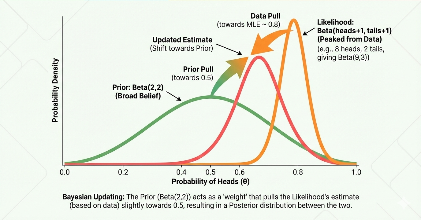
plt.show()

Maximum a Posteriori (MAP): Incorporating Priors

MAP extends MLE by including a prior distribution. It maximizes the posterior:

$\hat{\theta}_{MAP} = \arg\max_\theta P(\theta|X) = \arg\max_\theta P(X|\theta)P(\theta)$

Example: Estimating a probability with Beta prior

# Suppose we're estimating the probability of heads for a coin
# Prior: Beta(α=2, β=2) — slightly biased towards 0.5
α_prior, β_prior = 2, 2

# Data: 7 heads, 3 tails
heads, tails = 7, 3

# Posterior is Beta(α_prior + heads, β_prior + tails)
α_post = α_prior + heads
β_post = β_prior + tails

# MAP estimate is mode of Beta: (α-1)/(α+β-2) for α,β>1
map_estimate = (α_post - 1) / (α_post + β_post - 2)
mle_estimate = heads / (heads + tails)

print(f"MLE estimate: {mle_estimate:.3f}")
print(f"MAP estimate with Beta(2,2) prior: {map_estimate:.3f}")

# Visualize prior, likelihood, posterior
x = np.linspace(0, 1, 100)
plt.figure(figsize=(10, 6))
plt.plot(x, stats.beta.pdf(x, α_prior, β_prior), 'b-', label='Prior Beta(2,2)')
plt.plot(x, stats.beta.pdf(x, heads+1, tails+1), 'g--', label='Likelihood (MLE)')  # likelihood is Beta(heads+1, tails+1) for binomial
plt.plot(x, stats.beta.pdf(x, α_post, β_post), 'r-', label='Posterior Beta(9,5)')
plt.axvline(map_estimate, color='r', linestyle=':', label=f'MAP = {map_estimate:.3f}')
plt.axvline(mle_estimate, color='g', linestyle=':', label=f'MLE = {mle_estimate:.3f}')
plt.xlabel('θ (probability of heads)')
plt.ylabel('Density')
plt.title('Bayesian Inference: Prior → Likelihood → Posterior')
plt.legend()
plt.show()

Discriminative vs. Generative Models

This distinction is fundamental in ML:

• Discriminative models learn $P(y|x)$ directly — they draw boundaries between classes. Examples: logistic regression, SVMs, neural networks.
• Generative models learn $P(x,y)$ or $P(x|y)P(y)$ — they model how data is generated. Examples: Naive Bayes, GANs, VAEs.

Naive Bayes: A simple generative classifier

Naive Bayes assumes features are independent given the class:

$P(y|x_1,...,x_n) \propto P(y) \prod_{i=1}^n P(x_i|y)$

Despite its naive assumption, it works surprisingly well for text classification.

from sklearn.datasets import fetch_20newsgroups
from sklearn.feature_extraction.text import CountVectorizer
from sklearn.naive_bayes import MultinomialNB
from sklearn.metrics import classification_report

# Load a subset of newsgroups for speed
categories = ['alt.atheism', 'soc.religion.christian', 'comp.graphics', 'sci.med']
newsgroups = fetch_20newsgroups(subset='train', categories=categories)

# Convert text to bag-of-words
vectorizer = CountVectorizer(stop_words='english', max_features=1000)
X = vectorizer.fit_transform(newsgroups.data)
y = newsgroups.target

# Train Naive Bayes
clf = MultinomialNB()
clf.fit(X, y)

# Evaluate
X_test, y_test = fetch_20newsgroups(subset='test', categories=categories, return_X_y=True)
X_test = vectorizer.transform(X_test)
y_pred = clf.predict(X_test)
print(classification_report(y_test, y_pred, target_names=newsgroups.target_names))

Why is this generative? Because MultinomialNB learns $P(x_i|y)$ for each word and $P(y)$ — it models the process of generating documents.

Generative Models Beyond Naive Bayes

Modern generative models go much further:

• Gaussian Mixture Models (GMM): Assume data is generated from a mixture of Gaussians.
• Hidden Markov Models (HMM): For sequential data (speech, genomics).
• Variational Autoencoders (VAEs): Learn latent representations while modeling data distribution.
• Generative Adversarial Networks (GANs): Generate realistic images, audio, etc.

# Simple GMM example
from sklearn.mixture import GaussianMixture

# Generate data from two Gaussians
np.random.seed(42)
X1 = np.random.normal(0, 1, size=(200, 2))
X2 = np.random.normal(5, 1, size=(200, 2))
X = np.vstack([X1, X2])

# Fit GMM with 2 components
gmm = GaussianMixture(n_components=2)
gmm.fit(X)

# Predict component membership
labels = gmm.predict(X)

# Visualize
plt.figure(figsize=(8, 6))
plt.scatter(X[:, 0], X[:, 1], c=labels, cmap='viridis', alpha=0.6)
plt.title('Gaussian Mixture Model: Generative Clustering')
plt.show()

Conclusions

1. Probability quantifies uncertainty: ML models inherently deal with uncertainty, and probability gives us the tools to handle it.

2. Bayes’ theorem is the foundation of inference: It shows how to update beliefs with data — the essence of learning.

3. Distributions model data: Knowing which distribution fits your data (Gaussian for real-valued, Poisson for counts, etc.) guides model selection.

4. MLE and MAP are workhorses: Most ML training is essentially MLE or MAP with clever optimization.

5. Generative vs. discriminative: Understanding this distinction helps you choose the right tool: discriminative for prediction, generative for understanding data generation or handling missing data.

6. Modern deep generative models extend these ideas to high-dimensional data like images and text.

Real-World Applications

• Spam filtering: Naive Bayes
• Medical diagnosis: Bayesian networks
• Speech recognition: Hidden Markov Models
• Image generation: VAEs, GANs
• Recommendation systems: Probabilistic matrix factorization