Linear Algebra in ML From Matrices to Embeddings

Summary

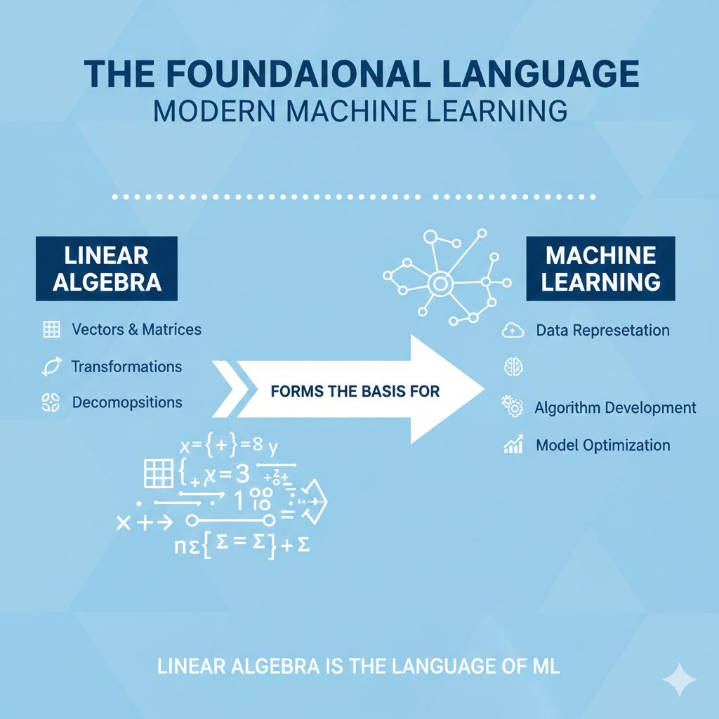
Linear algebra forms the fundamental language of modern machine learning. This article explores how seemingly abstract concepts—vectors, matrices, decompositions—materialize into practical applications ranging from dimensionality reduction to semantic representation learning.

Through concrete Python examples and intuitive analogies, we’ll discover how these mathematical tools enable models to process high-dimensional data, optimize operations, and capture complex relationships in domains like NLP and computer vision.

The Underlying Language of ML

At its core, machine learning is about finding patterns in data. Linear algebra provides the tools to represent and manipulate this data efficiently. Vectors and matrices allow us to encode features, relationships, and transformations in a structured way.

For instance, a dataset with multiple features can be represented as a matrix, where each row corresponds to a data point and each column corresponds to a feature. This representation enables us to perform operations like scaling, rotation, and projection, which are essential for tasks like dimensionality reduction and feature extraction.

In robotics, computer vision, and machine learning, every geometric transformation, data projection, and optimization operation has algebraic roots. When a recommendation system suggests products, when a classifier identifies images, or when a transformer processes language, they’re executing linear algebra operations massively and efficiently.

Fundamental Concepts with ML Applications

Vectors: More than Arrows in Space

Vectors are the building blocks of linear algebra. In machine learning, they represent data points, features, and even model parameters. For example, in a simple linear regression model, the weights can be represented as a vector that interacts with the input features to produce predictions.

In natural language processing (NLP), word embeddings are vectors that capture semantic relationships between words. The famous Word2Vec algorithm generates dense vector representations of words, where the distance between vectors reflects semantic similarity. For instance, the vector for “king” might be close to the vector for “queen,” while being far from the vector for “car.”

import numpy as np

# Classic analogy: king - man + woman = queen
embeddings = {
    "king": np.array([0.8, 0.1]),
    "queen": np.array([0.75, 0.15]),
    "man": np.array([0.1, -0.3]),
    "woman": np.array([0.15, 0.2])
}

# The algebraic magic of word2vec
analogy = embeddings["king"] - embeddings["man"] + embeddings["woman"]

# Find closest embedding (cosine similarity)
def cos_sim(a, b):
    return np.dot(a, b) / (np.linalg.norm(a) * np.linalg.norm(b))

for word, vector in embeddings.items():
    similarity = cos_sim(analogy, vector)
    print(f"Similarity with '{word}': {similarity:.3f}")

Matrices and Linear Transformations: The Heart of Neural Networks

Matrices are essential for representing linear transformations, which are at the core of neural networks. Each layer in a neural network can be thought of as a matrix that transforms the input data into a new space. For example, in a fully connected layer, the weights are represented as a matrix that multiplies the input vector to produce the output.

This transformation allows the network to learn complex patterns and relationships in the data. In convolutional neural networks (CNNs), the convolution operation can be represented as a matrix multiplication, where the filter is applied across the input image to extract features.

Just as homogeneous transformations in robotics concatenate operations (rotation + translation), neural networks stack linear transformations interleaved with nonlinearities, enabling modeling of complex relationships.

SVD Decomposition and PCA: Dimensionality Reduction and Feature Extraction

Singular Value Decomposition (SVD) is a powerful tool for dimensionality reduction and feature extraction. It decomposes a matrix into three components: $U$, $\Sigma$, and $V^T$. In machine learning, SVD is often used in Principal Component Analysis (PCA) to reduce the dimensionality of data while preserving as much variance as possible.

PCA identifies the directions (principal components) in which the data varies the most, allowing us to project high-dimensional data onto a lower-dimensional space. This is particularly useful for visualizing data, reducing noise, and improving the performance of machine learning models.

from sklearn.decomposition import PCA
import matplotlib.pyplot as plt

# Synthetic dataset: 100 samples, 50 features
np.random.seed(42)
X = np.dot(np.random.randn(100, 3), np.random.randn(3, 50))  # 3D latent structure

# PCA to find directions of maximum variance
pca = PCA(n_components=2)
X_pca = pca.fit_transform(X)

print(f"Variance explained by components: {pca.explained_variance_ratio_}")
print(f"Total preserved: {sum(pca.explained_variance_ratio_):.1%}")

# Visualization
plt.figure(figsize=(10, 8))
plt.scatter(X_pca[:, 0], X_pca[:, 1], alpha=0.7, edgecolors='k')
plt.xlabel('Principal Component 1', fontsize=12)
plt.ylabel('Principal Component 2', fontsize=12)
plt.title('PCA: Projection of High-Dimensional Data to 2D', fontsize=14)
plt.grid(True, alpha=0.3)
plt.show()

Computer vision application: In point cloud processing (as in pick-and-place systems), SVD is used to estimate object orientation by computing principal axes from the covariance matrix.

Tensors: Generalizing Linear Algebra to Higher Dimensions

Tensors are a generalization of vectors and matrices to higher dimensions. In machine learning, tensors are used to represent data with more than two dimensions, such as images (3D tensors) and videos (4D tensors). Deep learning frameworks like TensorFlow and PyTorch are built around tensor operations, allowing for efficient computation on GPUs.

Tensors enable us to perform complex operations like convolution, pooling, and backpropagation, which are essential for training deep neural networks. They also allow us to represent and manipulate data in a way that captures spatial and temporal relationships, making them crucial for tasks like image recognition and natural language processing.

import torch

# Common representations in ML
image_rgb = torch.randn(3, 224, 224)           # [channels, height, width]
batch_images = torch.randn(32, 3, 224, 224)    # [batch, channels, height, width]
text_sequence = torch.randn(10, 64, 300)       # [seq_length, batch, embedding_dim]

print(f"Image batch: {batch_images.shape}")
print(f"Text sequence: {text_sequence.shape}")

# Key operation: batched matrix multiplication
A = torch.randn(32, 10, 20)  # 32 matrices of 10×20
B = torch.randn(32, 20, 30)  # 32 matrices of 20×30
C = torch.bmm(A, B)          # 32 matrices of 10×30
print(f"Batched matmul result: {C.shape}")

Pseudo-inverse and Linear Systems: Solving Underdetermined and Overdetermined Problems

The pseudo-inverse is a generalization of the matrix inverse that allows us to solve linear systems that are either underdetermined (more variables than equations) or overdetermined (more equations than variables). In machine learning, the pseudo-inverse is used in linear regression to find the best-fitting line when the system of equations does not have a unique solution. It is also used in regularization techniques to prevent overfitting by adding a penalty term to the loss function.

By computing the pseudo-inverse of the design matrix, we can find the optimal weights for our model even when the data is noisy or when there are more features than samples.

# Example: polynomial fitting (overdetermined)
np.random.seed(123)
X = np.random.randn(100, 3)  # 100 samples, 3 features
y = 2*X[:,0] - 3*X[:,1] + 1.5*X[:,2] + np.random.randn(100)*0.1

# Least squares solution: w = (X^T X)^{-1} X^T y
# Using pseudoinverse (numerically stable)
X_pinv = np.linalg.pinv(X)  # Pseudoinverse via SVD
w = X_pinv @ y

print(f"Estimated coefficients: {w}")
print(f"Mean squared error: {np.mean((X @ w - y)**2):.6f}")

# Comparison with direct solution (less stable)
w_direct = np.linalg.inv(X.T @ X) @ X.T @ y
print(f"Difference between methods: {np.max(np.abs(w - w_direct)):.2e}")

Recommender systems: In collaborative filtering, the pseudo-inverse can be used to solve for user and item latent factors when the rating matrix is sparse, enabling predictions of missing ratings.

Conclusion

Linear algebra is the backbone of machine learning, providing the tools to represent and manipulate data in high-dimensional spaces. From the fundamental concepts of vectors and matrices to advanced techniques like SVD and tensor operations, linear algebra enables us to build powerful models that can learn from data and make predictions.

By understanding the linear algebraic foundations of machine learning, we can better appreciate the inner workings of algorithms and develop more efficient and effective models for a wide range of applications, from natural language processing to computer vision. As we continue to explore the frontiers of machine learning, the importance of linear algebra will only grow, making it an essential area of study for anyone interested in the field.