Calculus for ML: Gradients, Optimization and the Chain rule

Summary

If linear algebra provides the vocabulary of machine learning, calculus provides the grammar—it tells us how things change. This article demystifies the calculus concepts that power modern ML: derivatives for measuring change, gradients for multidimensional optimization, and the chain rule for training deep neural networks. Through intuitive explanations and practical Python examples, we’ll see how these mathematical tools enable models to learn from data, from simple linear regression to complex architectures like transformers.

Why Calculus is the Engine of Learning

Every time a machine learning model improves its predictions, it’s using calculus under the hood. The core idea is beautifully simple: learning is optimization, and optimization requires understanding how changes in parameters affect the final output.

Consider what happens during training:

A neural network makes a prediction (forward pass)
We calculate how wrong it was (loss function)
We need to adjust thousands or millions of parameters to reduce this error

Calculus gives us the tools to answer the critical question: “If I tweak this weight by a tiny amount, how much will the loss change?” This question—and its answer—is the foundation of gradient descent, backpropagation, and virtually all learning algorithms.

In robotics and simulation, calculus appears when we need to compute velocities from positions, accelerations from velocities, or optimize trajectories. The same mathematical principles govern how robots move and how neural networks learn.

Core Calculus Concepts with ML Applications

Derivatives: The Measure of Change

A derivative tells us how a function changes as its input changes. In ML terms: “If I increase this feature by a little, how much does my prediction change?”

import numpy as np
import matplotlib.pyplot as plt

# Simple example: linear regression prediction
def predict(X, w, b):
    return X * w + b

# Loss function: Mean Squared Error
def mse_loss(y_true, y_pred):
    return np.mean((y_true - y_pred) ** 2)

# Let's visualize how loss changes with weight
X = np.array([1, 2, 3, 4, 5])
y_true = np.array([2, 4, 6, 8, 10])  # Perfect line: y = 2x

# Try different weights
weights = np.linspace(0, 4, 100)
losses = []

for w in weights:
    y_pred = predict(X, w, b=0)
    losses.append(mse_loss(y_true, y_pred))

# Plot loss vs weight
plt.figure(figsize=(10, 6))
plt.plot(weights, losses, 'b-', linewidth=2)
plt.xlabel('Weight (w)', fontsize=12)
plt.ylabel('Loss', fontsize=12)
plt.title('How Loss Changes with Weight', fontsize=14)
plt.grid(True, alpha=0.3)
plt.axvline(x=2, color='r', linestyle='--', label='Optimal weight (w=2)')
plt.legend()
plt.show()

Partial Derivatives: Handling Multiple Dimensions

Real ML models have thousands or millions of parameters. Partial derivatives measure how the loss changes with respect to each parameter individually, holding others constant.

# Simple neural network with 2 inputs, 1 output
def simple_nn(X1, X2, w1, w2, b):
    """Simple neuron: y = sigmoid(w1*x1 + w2*x2 + b)"""
    z = w1 * X1 + w2 * X2 + b
    return 1 / (1 + np.exp(-z))  # Sigmoid activation

# Loss function: Binary Cross-Entropy
def bce_loss(y_true, y_pred):
    return -np.mean(y_true * np.log(y_pred) + (1 - y_true) * np.log(1 - y_pred))

# Sample data point
x1, x2 = 2.0, 3.0
y_true = 1.0

# Current parameters
w1, w2, b = 0.5, -0.3, 0.1

# Forward pass
y_pred = simple_nn(x1, x2, w1, w2, b)
loss = bce_loss(y_true, y_pred)

print(f"Prediction: {y_pred:.4f}, Loss: {loss:.4f}")

# To improve, we need ∂loss/∂w1, ∂loss/∂w2, ∂loss/∂b
# These partial derivatives tell us how to adjust each parameter

The Chain Rule: The Heart of Deep Learning

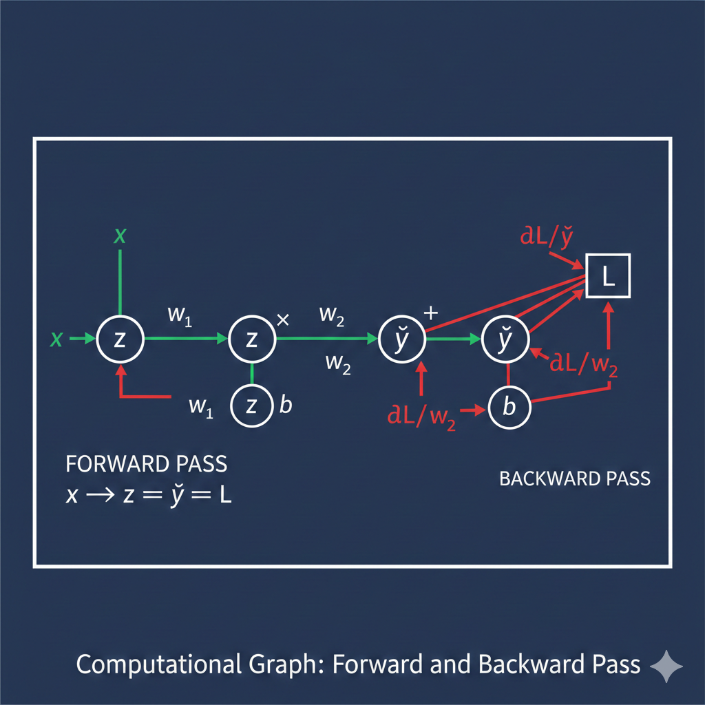
The chain rule allows us to compute derivatives through composite functions—exactly what we need when propagating errors through neural network layers.

If we have a function composition $y = f(g(x))$ , the chain rule states:

$dy/dx = (df/dg) * (dg/dx)$

In neural networks, this becomes a cascade:

Loss depends on prediction
Prediction depends on hidden layer outputs
Hidden layer outputs depend on weights

Step-by-step derivation for a classification perceptron:

For a binary classification problem with sigmoid activation and log loss, we have:

Forward pass:
- $z = w₁x₁ + w₂x₂ + b$
- $ŷ = σ(z) = 1/(1 + e⁻ᶻ)$
- $L = -[y log(ŷ) + (1-y) log(1-ŷ)]$
We need $∂L/∂w₁$ , $∂L/∂w₂$ , and $∂L/∂b$ for gradient descent
Using the chain rule:
- $∂L/∂w₁ = (∂L/∂ŷ) × (∂ŷ/∂z) × (∂z/∂w₁)$
Computing each piece:
- $∂L/∂ŷ = -(y/ŷ - (1-y)/(1-ŷ))$ (derivative of log loss)
- $∂ŷ/∂z = ŷ(1-ŷ)$ (derivative of sigmoid)
- $∂z/∂w₁ = x₁$
Multiplying and simplifying gives us the elegant result:
- $∂L/∂w₁ = (ŷ - y) × x₁$
- $∂L/∂b = ŷ - y$

This is remarkably simple! The gradient is just the prediction error times the input.

# Implementing what we just derived
def compute_gradients(x1, x2, y_true, w1, w2, b):
    # Forward pass
    z = w1 * x1 + w2 * x2 + b
    y_pred = 1 / (1 + np.exp(-z))
    
    # Gradients (using our derived formulas!)
    error = y_pred - y_true
    grad_w1 = error * x1
    grad_w2 = error * x2
    grad_b = error
    
    return grad_w1, grad_w2, grad_b, y_pred

# Test it
x1, x2, y_true = 2.0, 3.0, 1.0
w1, w2, b = 0.5, -0.3, 0.1

grad_w1, grad_w2, grad_b, y_pred = compute_gradients(x1, x2, y_true, w1, w2, b)

print(f"Prediction: {y_pred:.4f}")
print(f"Gradients: ∂L/∂w₁ = {grad_w1:.4f}, ∂L/∂w₂ = {grad_w2:.4f}, ∂L/∂b = {grad_b:.4f}")
print(f"Interpretation: {'Increase' if grad_w1 < 0 else 'Decrease'} w₁ by {abs(grad_w1):.4f}")

Gradient Descent: Putting It All Together

Gradient descent uses these partial derivatives to iteratively improve parameters:

def gradient_descent_step(x1, x2, y_true, w1, w2, b, learning_rate=0.1):
    # Compute gradients
    grad_w1, grad_w2, grad_b, y_pred = compute_gradients(x1, x2, y_true, w1, w2, b)
    
    # Update parameters (descend the gradient)
    w1_new = w1 - learning_rate * grad_w1
    w2_new = w2 - learning_rate * grad_w2
    b_new = b - learning_rate * grad_b
    
    return w1_new, w2_new, b_new, y_pred

# Train on a single point
x1, x2, y_true = 2.0, 3.0, 1.0
w1, w2, b = 0.0, 0.0, 0.0  # Start from zero

print("Training on one data point:")
print(f"{'Step':<5} {'w₁':<10} {'w₂':<10} {'b':<10} {'ŷ':<10} {'Loss':<10}")
print("-" * 55)

for step in range(10):
    w1, w2, b, y_pred = gradient_descent_step(x1, x2, y_true, w1, w2, b, learning_rate=0.5)
    loss = - (y_true * np.log(y_pred + 1e-15) + (1-y_true) * np.log(1 - y_pred + 1e-15))
    print(f"{step:<5} {w1:<10.4f} {w2:<10.4f} {b:<10.4f} {y_pred:<10.4f} {loss:<10.4f}")

Advanced: Gradients, Jacobians, and Hessians

As models grow more complex, so do our calculus tools:

Gradient: Vector of all partial derivatives $∇L = [∂L/∂θ₁, ∂L/∂θ₂, ..., ∂L/∂θₙ]$
Jacobian: Matrix of all first-order derivatives for vector-valued functions
Hessian: Matrix of second-order derivatives, capturing curvature information

# In PyTorch, automatic differentiation handles all of this
import torch

# Create tensors with gradient tracking
x1 = torch.tensor(2.0, requires_grad=True)
x2 = torch.tensor(3.0, requires_grad=True)
w1 = torch.tensor(0.5, requires_grad=True)
w2 = torch.tensor(-0.3, requires_grad=True)
b = torch.tensor(0.1, requires_grad=True)
y_true = torch.tensor(1.0)

# Forward pass
z = w1 * x1 + w2 * x2 + b
y_pred = torch.sigmoid(z)
loss = - (y_true * torch.log(y_pred) + (1 - y_true) * torch.log(1 - y_pred))

# Backward pass (automatic differentiation!)
loss.backward()

# Gradients are automatically computed!
print(f"PyTorch gradients:")
print(f"  ∂L/∂w₁ = {w1.grad.item():.4f}")
print(f"  ∂L/∂w₂ = {w2.grad.item():.4f}")
print(f"  ∂L/∂b = {b.grad.item():.4f}")

# Compare with our manual calculation
error = y_pred.item() - y_true.item()
print(f"\nManual calculation:")
print(f"  ∂L/∂w₁ = {error * x1.item():.4f}")
print(f"  ∂L/∂w₂ = {error * x2.item():.4f}")
print(f"  ∂L/∂b = {error:.4f}")

Integrals and Their ML Applications

While derivatives get most of the attention, integrals appear in important ML contexts:

ROC-AUC: Area under the ROC curve measures model performance
Probability distributions: Continuous probabilities require integration
Expected values: Many loss functions involve expectations over distributions

from sklearn.metrics import roc_curve, auc
import matplotlib.pyplot as plt

# Sample predictions and true labels
y_true = np.array([0, 0, 1, 1, 0, 1, 0, 1, 1, 0])
y_scores = np.array([0.1, 0.2, 0.8, 0.7, 0.3, 0.9, 0.2, 0.6, 0.85, 0.15])

# Compute ROC curve
fpr, tpr, thresholds = roc_curve(y_true, y_scores)
roc_auc = auc(fpr, tpr)  # This is an integral!

# Visualize
plt.figure(figsize=(8, 6))
plt.plot(fpr, tpr, 'b-', linewidth=2, label=f'ROC curve (AUC = {roc_auc:.3f})')
plt.plot([0, 1], [0, 1], 'r--', label='Random classifier')
plt.xlabel('False Positive Rate', fontsize=12)
plt.ylabel('True Positive Rate', fontsize=12)
plt.title('ROC Curve: Integration in Model Evaluation', fontsize=14)
plt.legend()
plt.grid(True, alpha=0.3)
plt.show()

print(f"Area Under the Curve (AUC): {roc_auc:.3f}")
print(f"This AUC value comes from integrating the ROC curve!")

Conclusions

Calculus quantifies change: Derivatives tell us how adjusting any parameter will affect our model’s performance.
The chain rule enables deep learning: By decomposing complex functions, we can compute gradients through hundreds of layers efficiently.
Gradient descent is learning: The simple idea of “follow the negative gradient” is responsible for training virtually every ML model.
Automatic differentiation handles complexity: Modern frameworks like PyTorch and TensorFlow implement these calculus concepts so we can focus on model architecture.
Integrals matter too: From probability to model evaluation, integration plays a crucial role in ML workflows.

Real-World Applications

Finance: Derivatives for risk modeling, optimization for portfolio allocation
Healthcare: Differential equations for disease modeling, gradients for medical image analysis
Robotics: Calculus for trajectory optimization, control systems, and sensor fusion